Species richness estimation

This is a basic workflow for feeding species occurrence data, a group’s taxonomy, and a group’s country checklist into BeeBDC in order to produce species richness estimates. Some of these functions are also generic wrappers around SpadeR and iNEXT functions that can be used with any abundance data. These functions have grown from an original publication.

Script preparation

Working directory

Choose the path to the root folder in which all other folders can be found.

RootPath <- paste0("/your/path/here")

# Create the working directory in the RootPath if it doesn't exist already
if (!dir.exists(paste0(RootPath, "/Data_acquisition_workflow"))) {
    dir.create(paste0(RootPath, "/Data_acquisition_workflow"), recursive = TRUE)
}
# Set the working directory
setwd(paste0(RootPath, "/Data_acquisition_workflow"))

Install packages (if needed)

You may need to install some packages for using this workflow. In particular, SpadeR and iNEXT are required. They should prompt you to download them the first time that you run the functions, however, let’s install them here and now.

install.packages("SpadeR")
install.packages("iNEXT")

Parallel estimations

We can start by looking at the relatively simple iNEXT and SpadeR wrapper functions that can take the usual inputs for those functions in their host packages. (See iNEXT::iNEXT() and SpadeR::ChaoSpecies() for more info.) These functions can take your data and run multiple sites/countries/whatever level you want to throw at them and run them in parallel. This greatly simplifies the code needed to run them and also makes its implementation MUCH faster!

iNEXTwrapper

BeeBDC::iNEXTwrapper() parallelizes iNEXT::iNEXT(), which estimates species richness patterns by extrapolating and interpolating Hill numbers. By and large this kinda equates to estimating richness by rarefaction. We can start by reading in an example dataset with 1,488 scientificName-country_suggested combinations across four countries; Fiji, Uganda, Vietnam, and Zambia.

beesCountrySubset <- BeeBDC::beesCountrySubset

Next, let’s look at how we would usually use iNEXT… By first transforming our (very simple example) occurrence dataset into the right format and then running the function.

# Transform the data
transformedAbundance <- beesCountrySubset %>%
    dplyr::group_by(scientificName, country_suggested) %>%
    dplyr::count() %>%
    dplyr::select(scientificName, country_suggested, n) %>%
    tidyr::pivot_wider(names_from = country_suggested, values_from = n, values_fill = 0) %>%
    # Create the rownames
tibble::column_to_rownames("scientificName") %>%
    dplyr::tibble() %>%
    as.data.frame()
# Run iNEXT
output_iNEXT <- iNEXT::iNEXT(transformedAbundance, datatype = "abundance")

We can also view the output of this function by running output_iNEXT$AsyEst

Assemblage	Diversity	Observed	Estimator	s.e.	LCL	UCL
Fiji	Species richness	17.000000	17.499483	1.4850098	17.000000	20.410049
Fiji	Shannon diversity	4.712056	4.754101	0.2164397	4.329887	5.178315
Fiji	Simpson diversity	2.653013	2.657561	0.1237356	2.415044	2.900078
Uganda	Species richness	44.000000	70.243359	14.1752423	44.000000	98.026324
Uganda	Shannon diversity	19.651483	26.633143	3.4844763	19.803695	33.462591
Uganda	Simpson diversity	7.699248	8.128000	1.5689856	5.052845	11.203155
Vietnam	Species richness	6.000000	13.794872	5.8924098	6.000000	25.343783
Vietnam	Shannon diversity	1.953128	2.307552	0.5923478	1.146572	3.468532
Vietnam	Simpson diversity	1.386509	1.400756	0.1986146	1.011479	1.790034
Zambia	Species richness	129.000000	186.853965	17.7824798	152.000945	221.706985
Zambia	Shannon diversity	77.832700	104.647375	7.6001195	89.751415	119.543336
Zambia	Simpson diversity	32.753790	35.991359	6.3494595	23.546647	48.436071

The implementation of BeeBDC::iNEXTwrapper() is also relatively simple; including the implementation of running in parallel (Note: Windows machines can’t use R’s parallel functions). We can again modify the input data to work with the function as below and we could leave most of the inputs to iNEXTwrapper to the defaults or change them as we saw fit. The key variable is to change mc.cores to however many threads you’d liek to use on your computer!

# Transform data
data_nextWrapper <- beesCountrySubset %>%
    dplyr::group_by(scientificName, country_suggested) %>%
    dplyr::count()

# Calculate iNEXT with the wrapper function
output_iNEXTwrapper <- BeeBDC::iNEXTwrapper(data = data_nextWrapper, variableColumn = "country_suggested",
    valueColumn = "n", q = 0, datatype = "abundance", conf = 0.95, se = TRUE, nboot = 50,
    size = NULL, endpoint = NULL, knots = 40, mc.cores = 1)

##  - Outputs can be found in a list with two tibbles called 'DataInfo' and 'AsyEst' and a list of iNext outputs per groupVariable in iNextEst'.

country_suggested	statistic	Observed	Estimator	Est_s.e.	95% Lower	95% Upper
Fiji	Species Richness	17.000000	17.499483	1.6650163	14.236111	20.762855
Fiji	Shannon diversity	4.712056	4.754101	0.2271829	4.308831	5.199372
Fiji	Simpson diversity	2.653013	2.657561	0.1264695	2.409685	2.905436
Uganda	Species Richness	44.000000	70.243359	25.7541584	19.766137	120.720582
Uganda	Shannon diversity	19.651483	26.633143	4.2573468	18.288896	34.977389
Uganda	Simpson diversity	7.699248	8.128000	1.8631187	4.476354	11.779646
Vietnam	Species Richness	6.000000	13.794872	6.1393736	1.761921	25.827823
Vietnam	Shannon diversity	1.953128	2.307552	0.5633747	1.203358	3.411746
Vietnam	Simpson diversity	1.386509	1.400756	0.1830418	1.042001	1.759511
Zambia	Species Richness	129.000000	186.853965	18.1990609	151.184461	222.523469
Zambia	Shannon diversity	77.832700	104.647375	6.8285323	91.263698	118.031053
Zambia	Simpson diversity	32.753790	35.991359	5.5923079	25.030637	46.952081

ChaoWrapper

BeeBDC::ChaoWrapper() parallelizes SpadeR::ChaoSpecies(), which estimates species richness using various non-parametric estimators. The primary one that I tend to use is iChao. Let’s use the same example dataset to first run the SpadeR function.

# Transform data
data_iChao <- beesCountrySubset %>%
    dplyr::group_by(scientificName, country_suggested) %>%
    dplyr::count() %>%
    dplyr::select(scientificName, country_suggested, n) %>%
    tidyr::pivot_wider(names_from = country_suggested, values_from = n, values_fill = 0) %>%
    # Create the rownames
tibble::column_to_rownames("scientificName") %>%
    dplyr::tibble()

# Run ChaoSpecies for the country Fiji
output_iChao <- SpadeR::ChaoSpecies(data_iChao$Fiji, datatype = "abundance")

Let’s view the output of this function by running output_iChao$Species_table. Once again, you’ll be able to see that there are actually quite a few species richness estimators available here.

	Estimate	s.e.	95%Lower	95%Upper
Homogeneous Model	17.182	0.474	17.011	20.015
Homogeneous (MLE)	17.000	0.633	17.000	18.858
Chao1 (Chao, 1984)	17.499	1.322	17.030	25.434
Chao1-bc	17.000	0.633	17.000	18.858
iChao1 (Chiu et al. 2014)	17.624	1.322	17.048	25.048
ACE (Chao & Lee, 1992)	17.342	0.775	17.024	21.788
ACE-1 (Chao & Lee, 1992)	17.366	0.835	17.026	22.168
1st order jackknife	17.999	1.413	17.128	24.796
2nd order jackknife	18.000	2.446	17.065	32.367

The implementation of the parallel wrapper is also quite simple for BeeBDC::ChaoWrapper(). And the number of cores can also be changed using the mc.cores argument. Note, that in this case, we can run all sites (or countries) at once!

# Run the wrapper function
output_iChaowrapper <- BeeBDC::ChaoWrapper(data = data_iChao, datatype = "abundance",
    k = 10, conf = 0.95, mc.cores = 1)

##  - Outputs can be found in a list with two tibbles called 'basicTable' and 'richnessTable'.

View the output with output_iChaowrapper$richnessTable.

variable	Name	Estimate	s.e.	95%Lower	95%Upper
Zambia	Homogeneous Model	159.936	8.471	147.263	181.402
Zambia	Homogeneous (MLE)	140.234	3.957	134.748	150.959
Zambia	Chao1 (Chao, 1984)	186.854	20.305	158.664	241.834
Zambia	Chao1-bc	183.879	19.243	157.155	235.970
Zambia	iChao1 (Chiu et al. 2014)	199.091	12.645	178.353	228.541
Zambia	ACE (Chao & Lee, 1992)	183.240	15.921	159.876	224.286
Zambia	ACE-1 (Chao & Lee, 1992)	197.138	22.684	165.093	257.634
Zambia	1st order jackknife	185.839	10.654	168.488	210.814
Zambia	2nd order jackknife	214.754	18.422	185.553	259.032
Uganda	Homogeneous Model	59.952	7.062	50.961	80.554
Uganda	Homogeneous (MLE)	47.113	2.032	44.969	54.004
Uganda	Chao1 (Chao, 1984)	70.243	14.659	53.450	116.878
Uganda	Chao1-bc	66.820	12.672	52.261	107.041
Uganda	iChao1 (Chiu et al. 2014)	76.243	8.394	63.519	97.262
Uganda	ACE (Chao & Lee, 1992)	78.927	16.764	58.308	129.256
Uganda	ACE-1 (Chao & Lee, 1992)	95.184	30.929	61.149	196.767
Uganda	1st order jackknife	66.820	6.743	56.944	84.233
Uganda	2nd order jackknife	79.695	11.623	63.160	110.499
Fiji	Homogeneous Model	17.182	0.474	17.011	20.015
Fiji	Homogeneous (MLE)	17.000	0.633	17.000	18.858
Fiji	Chao1 (Chao, 1984)	17.499	1.322	17.030	25.434
Fiji	Chao1-bc	17.000	0.633	17.000	18.858
Fiji	iChao1 (Chiu et al. 2014)	17.624	1.322	17.048	25.048
Fiji	ACE (Chao & Lee, 1992)	17.342	0.775	17.024	21.788
Fiji	ACE-1 (Chao & Lee, 1992)	17.366	0.835	17.026	22.168
Fiji	1st order jackknife	17.999	1.413	17.128	24.796
Fiji	2nd order jackknife	18.000	2.446	17.065	32.367
Vietnam	Homogeneous Model	16.000	12.450	7.501	72.612
Vietnam	Homogeneous (MLE)	6.009	0.096	6.000	6.644
Vietnam	Chao1 (Chao, 1984)	13.795	11.372	6.961	69.218
Vietnam	Chao1-bc	8.923	4.085	6.380	28.471
Vietnam	iChao1 (Chiu et al. 2014)	13.795	11.372	6.961	69.218
Vietnam	ACE (Chao & Lee, 1992)	16.000	12.450	7.501	72.612
Vietnam	ACE-1 (Chao & Lee, 1992)	16.000	12.450	7.501	72.612
Vietnam	1st order jackknife	9.897	2.774	7.111	19.668
Vietnam	2nd order jackknife	12.769	4.734	7.965	29.318

Visualising

These are both easy and simple to use wrapper functions. However, the complexity of the output data types can actually be a little bit confusing to work with. Especially if you want to visualise those data. So, we also provide the function, BeeBDC::ggRichnessWrapper() to display the results of both wrapper functions by site. Not only does this functino save a plot that visualises the data (below), it also outputs a summary of the estimates.

(plot_summary <- BeeBDC::ggRichnessWrapper(iNEXT_in = output_iNEXTwrapper, iChao_in = output_iChaowrapper,
    nrow = 2, ncol = 2, labels = NULL, fileName = "speciesRichnessPlots", outPath = tempdir(),
    base_width = 8.3, base_height = 11.7, dpi = 300))

## Loading required namespace: cowplot

## # A tibble: 4 × 11
##   level       n observedRichness iNEXT_est iNEXT_lower iNEXT_upper
##   <chr>   <dbl>            <dbl>     <dbl>       <dbl>       <dbl>
## 1 Fiji      967               17        17          14          21
## 2 Uganda    128               44        70          20         121
## 3 Vietnam    39                6        14           2          26
## 4 Zambia    354              129       187         151         223
## # ℹ 5 more variables: iNEXT_increasePercent <dbl>, iChao_est <dbl>,
## #   iChao_lower <dbl>, iChao_upper <dbl>, iChao_increasePercent <dbl>

Note that Fiji’s diversity seems to be reaching asymptote, but the remaining country’s species richnesses are still climbing. Vietnam in particular has a huge amount of uncertainty with the iChao estimates (green) reaching over 60 species! We knew that this was a really small dataset (in fact we chose it as a test dataset because it is small), but it goes to show that if your data are inadequate you may not get a great answer. On the plus side, the 95% confidence intervals all overlap.

level	n	observedRichness	iNEXT_est	iNEXT_lower	iNEXT_upper	iNEXT_increasePercent	iChao_est	iChao_lower	iChao_upper	iChao_increasePercent
Fiji	967	17	17	14	21	2.85	18	17	25	3.54
Uganda	128	44	70	20	121	37.36	76	64	97	42.29
Vietnam	39	6	14	2	26	56.51	14	7	69	56.51
Zambia	354	129	187	151	223	30.96	199	178	229	35.21

You can see, that these functions are moving towards simplifying quick and mass-estimation of species richness across sites or countries! The is the idea behind these improvements. But, we take this further below by also attempting to sample known taxa that are otherwise missing from our datasets!

Estimating richness from the known unknowns

Seems like a bit of an odd title, no? Well, many taxa have country-level checklists. Even insect taxa can be well represented in global country-level checklists; for example, ants, butterflies, dragonflies, and bees. While for vertebrates the situation is even better. Country-level global checklists often incorporate knowledge that isn’t contianed in species occurrence datasets but that, perhaps, we can take advantage of.

Preparing the inputs

In our bee species richness estimates paper, we had 4,819 species (from a total of ~21,000 species) that had no occurrence records globally. We could have run the above species richness estimates using just the occurrences that we had, but we wanted to incorporate that knowledge in our estimates. To do so, we found the samples sizes from most-recent literature for 497 species and generated a curve (we also generated this curve using the global- and country-level occurrence datasets and found the former to match the literature curve well).

Curves generated using 497 literature species (yellow), the global occurrence records (light blue), and occurrences at the country-level (dark blue).

We can then extract the formula from this curve and use it to randomly generate data for those missing species. These curves can be built using your own data; see section 1.6 of the R code for the bee species richness estimates paper, which uses ggplot2 and mosaic’s fitModel function to generate the curve function that goes into BeeBDC::diversityPrepR() below.

Let’s dig in… To start with, we will make an R object using our occurrence data (beesCountrySubset), taxonomy (from BeeBDC::beesTaxonomy() or BeeBDC::taxadbToBeeBDC()), and country checklist(BeeBDC::beesChecklist() or a manually-made checklist with the countries in the rNaturalEarth_name column and species in the validName column; the latter must match the remaining data — see BeeBDC::HarmoniseR()). Feel free to explore the input files or the output list of files for modifying your own and pay attention to match the column names.

Note as well that the curveFunction is the one generated from the Literature curve above.

# Download the taxonomy and checklist files
taxonomyFile <- BeeBDC::beesTaxonomy()
checklistFile <- BeeBDC::beesChecklist()

  # Generate the R file
estimateData <- BeeBDC::richnessPrepR(
  data = beesCountrySubset,
    # Download the bee taxonomy. Download other taxonomies using BeeBDC::taxadbToBeeBDC()
  taxonomyFile = taxonomyFile,
    # Download the bee country checklist. See notes above about making a checklist for other taxa
  checklistFile = checklistFile,
  curveFunction = function(x) (228.7531 * x * x^-log(12.1593)),
  sampleSize = 10000,
  countryColumn = "country_suggested"
)

Making estimates

The output file from the above code is then used to feed into the BeeBDC::richnessEstimator() function which will repeatedly sample the provided curve and estimate species richness (a user-defined number of times) at the country (or site), continental, or global level. This function can also be run in parallel and run at whatever scale the user asks for. If globalSamples, continentSamples, or countrySamples are set to zero, they will not be run. If they are set to >0, they will be estimated that many times. Let’s run our estimates at the country (or site) level ten times below, drawing sample sizes from the non-occurrence species each time (capped at the maximum sample size for each country).

estimates <- BeeBDC::richnessEstimateR(
  data = estimateData,
  sampleSize = 10000,
  globalSamples = 0,
  continentSamples = 0,
  countrySamples = 10,
    # Increase the number of cores to use R's parallel package and speed estimates up.
  mc.cores = 1,
    # Directory where to save files
  outPath = tempdir(),
  fileName = "Sampled.pdf"
)

We can look at the median outputs of our analysis with estimates$Summary.

name	scale	nChao	iChao_est	iChao_lower	iChao_upper	observedRichness	level	niNEXT	iNEXT_est	iNEXT_lower	iNEXT_upper	iNEXT_increasePercent	iNEXT_increase	iChao_increasePercent	iChao_increase
Fiji	Country	1069.5	41.2800	35.7385	64.478	33	Country	1069.5	40.13962	18.00921	63.07683	21.63521	7.139619	25.09091	8.2800
Vietnam	Country	543.0	194.9365	164.5450	243.644	114	Country	543.0	182.49250	136.45773	227.28721	60.08114	68.492501	70.99693	80.9365
Zambia	Country	878.0	348.9450	320.1285	384.994	227	Country	878.0	325.93280	280.62542	370.11176	43.58273	98.932797	53.72026	121.9450
Uganda	Country	1107.0	405.0855	360.8960	466.098	235	Country	1107.0	378.01122	320.83263	437.07824	60.85584	143.011221	72.37681	170.0855

Or, we can look at the outputs from each iteration together with estimates$SiteOutput.

variable	Name	Observed	Estimate	s.e.	95%Lower	95%Upper	n	groupNo
Fiji	iNEXT	33	35.49759	5.134940	25.433294	45.56189	1038	1
Fiji	iChao	NA	35.49800	2.956000	33.399000	48.63300	1038	1
Fiji	iNEXT	33	37.49583	6.700685	24.362732	50.62893	1080	1
Fiji	iChao	NA	40.61900	3.812000	36.017000	52.24000	1051	1
Fiji	iNEXT	33	39.11941	6.890805	25.613683	52.62514	1096	1
Fiji	iNEXT	33	37.49575	9.744875	18.396147	56.59535	1059	1
Fiji	iChao	NA	37.49600	4.798000	33.814000	57.83400	1059	1
Fiji	iChao	NA	37.49600	4.798000	33.814000	57.83500	1080	1
Fiji	iNEXT	33	39.11917	10.968008	17.622271	60.61607	1051	1
Fiji	iChao	NA	39.86900	6.073000	34.549000	63.46200	1096	1
Fiji	iChao	NA	41.94100	6.586000	35.460000	65.49400	1194	1
Fiji	iNEXT	33	41.15983	12.437858	16.782073	65.53758	1194	1
Fiji	iNEXT	33	46.48758	12.294538	22.390729	70.58443	1087	1
Fiji	iChao	NA	49.86300	8.194000	39.839000	74.57500	1087	1
Fiji	iNEXT	33	49.65139	18.836939	12.731669	86.57111	1091	1
Fiji	iNEXT	33	57.97535	24.305222	10.337985	105.61271	1014	1
Fiji	iChao	NA	53.15100	14.832000	38.550000	106.17400	1091	1
Fiji	iChao	NA	61.97500	20.732000	41.218000	135.16600	1014	1
Fiji	iNEXT	33	68.96418	34.599175	1.151042	136.77732	1005	1
Vietnam	iChao	NA	165.51800	10.908000	148.175000	191.66300	402	1
Fiji	iChao	NA	75.71400	33.374000	44.040000	198.26000	1005	1
Vietnam	iNEXT	114	162.87811	20.046949	123.586812	202.16941	402	1
Vietnam	iNEXT	114	171.68745	18.819271	134.802355	208.57254	616	1
Vietnam	iNEXT	114	169.13387	20.300560	129.345503	208.92224	606	1
Vietnam	iChao	NA	182.63400	13.906000	160.324000	215.68700	606	1
Vietnam	iNEXT	114	178.24875	20.373287	138.317845	218.17966	487	1
Vietnam	iChao	NA	184.81200	14.299000	161.856000	218.78100	616	1
Vietnam	iNEXT	114	178.86955	23.459225	132.890309	224.84878	643	1
Vietnam	iNEXT	114	188.91401	20.822637	148.102396	229.72563	640	1
Vietnam	iChao	NA	188.62400	17.139000	161.850000	230.37900	487	1
Vietnam	iNEXT	114	187.78641	25.343983	138.113112	237.45970	549	1
Vietnam	iChao	NA	190.75800	19.053000	161.532000	237.95500	643	1
Vietnam	iNEXT	114	193.86232	23.915989	146.987845	240.73680	468	1
Vietnam	iNEXT	114	186.11546	29.121147	129.039057	243.19186	537	1
Vietnam	iNEXT	114	196.69344	24.457159	148.758288	244.62859	442	1
Vietnam	iChao	NA	199.11500	20.424000	167.532000	249.33300	537	1
Vietnam	iChao	NA	205.57500	19.181000	175.010000	251.45400	549	1
Vietnam	iChao	NA	202.85600	21.714000	169.422000	256.45900	442	1
Vietnam	iChao	NA	204.65000	21.625000	171.162000	257.75600	640	1
Vietnam	iChao	NA	204.23700	24.744000	167.234000	266.96100	468	1
Zambia	iNEXT	227	313.16328	25.061705	264.043237	362.28332	888	1
Zambia	iChao	NA	333.18600	14.379000	308.531000	365.29700	888	1
Zambia	iNEXT	227	320.89257	22.663955	276.472037	365.31311	875	1
Zambia	iNEXT	227	320.91149	23.510925	274.830925	366.99206	946	1
Zambia	iNEXT	227	324.98214	22.282161	281.309912	368.65438	848	1
Zambia	iNEXT	227	322.91332	23.398235	277.053623	368.77302	991	1
Zambia	iNEXT	227	326.88345	22.738714	282.316388	371.45051	789	1
Uganda	iNEXT	235	329.10019	22.843495	284.327762	373.87262	1097	1
Zambia	iChao	NA	339.63400	16.516000	311.628000	376.90800	875	1
Zambia	iChao	NA	340.04500	16.610000	311.889000	377.53900	946	1
Zambia	iNEXT	227	329.28571	25.176376	279.940925	378.63050	896	1
Zambia	iChao	NA	344.35800	16.234000	316.603000	380.71000	991	1
Zambia	iChao	NA	346.96200	16.559000	318.644000	384.03000	848	1
Zambia	iNEXT	227	339.25597	22.972102	294.231474	384.28046	837	1
Zambia	iChao	NA	350.92800	15.804000	323.618000	385.95800	789	1
Uganda	iChao	NA	351.34000	16.547000	323.160000	388.52800	1097	1
Zambia	iChao	NA	351.76800	17.700000	321.613000	391.53500	896	1
Uganda	iNEXT	235	338.99729	26.807594	286.455375	391.53921	1101	1
Uganda	iChao	NA	364.95200	15.484000	337.971000	399.00300	1101	1
Zambia	iChao	NA	361.11400	20.731000	326.237000	408.25000	837	1
Uganda	iNEXT	235	368.61930	26.656869	316.372797	420.86581	938	1
Uganda	iNEXT	235	363.84466	32.199756	300.734297	426.95502	1113	1
Uganda	iNEXT	235	370.89746	29.746222	312.595935	429.19898	1179	1
Zambia	iNEXT	227	371.69757	29.856021	313.180845	430.21430	752	1
Uganda	iNEXT	235	385.12498	30.527359	325.292459	444.95751	1146	1
Uganda	iChao	NA	388.63500	24.798000	347.198000	445.37700	1113	1
Uganda	iChao	NA	396.90900	23.951000	356.349000	451.02600	938	1
Uganda	iChao	NA	397.83900	25.575000	354.919000	456.12100	1179	1
Zambia	iChao	NA	397.75200	26.418000	353.313000	457.82600	752	1
Zambia	iNEXT	227	392.04774	34.529010	324.372125	459.72335	881	1
Uganda	iNEXT	235	396.83960	33.621842	330.942006	462.73720	1010	1
Uganda	iChao	NA	412.33200	27.956000	365.443000	476.07500	1146	1
Uganda	iNEXT	235	404.38762	39.128240	327.697680	481.07756	1036	1
Zambia	iChao	NA	416.90200	33.509000	361.736000	494.65600	881	1
Uganda	iChao	NA	422.00200	32.524000	368.323000	497.29400	1010	1
Uganda	iNEXT	235	427.36223	42.028301	344.988270	509.73618	1255	1
Uganda	iChao	NA	441.38800	31.271000	388.619000	512.28200	1036	1
Uganda	iChao	NA	464.35200	39.795000	398.646000	556.44000	1255	1
Uganda	iNEXT	235	524.96190	56.241033	414.731501	635.19230	1196	1
Uganda	iChao	NA	556.33300	71.962000	443.284000	730.74000	1196	1

Visualising estimates

Of course, these values are super helpful for papers on these topics. But similarly, we can easily make some further useful visualisations!

# To build the manual legend, make a small fake dataset
legendData <- dplyr::tibble(name = c("yes","yes"),
                                              statistic = c("iChao", "iNEXT") %>%
                                                factor(levels = c("iChao", "iNEXT")),
                                              est = c(1,1))
# Build a legend manually
violinLegend <- ggplot2::ggplot(legendData, ggplot2::aes(x = name, y = est)) + 
  ggplot2::geom_point(data = legendData, ggplot2::aes(y=est, x = name, colour = "red")) + 
   scale_color_manual(labels = c('Observed'), values = c('grey30'))  +
   ggplot2::geom_bar(aes(fill = statistic, y = est), position = position_dodge(0.90),  
                     stat = "identity") +
   ggplot2::scale_fill_manual(name = "Statistic",
                              labels = c("iChao", "iNEXT"),
                              values = c("iChao" = "#55AD9B", "iNEXT" = "#FD9B63")) +
   ggplot2::theme_classic() +
   theme(legend.title = element_blank(), legend.position = 'right', 
         legend.margin = margin(0, 0, 0, 0), legend.spacing.y = unit(0, "pt")) +
   ggplot2::guides(fill = ggplot2::guide_legend(ncol = 1, byrow = TRUE, reverse = TRUE, order = 1))

# plot the countries 
(violinPlot <- ggplot2::ggplot(estimates$SiteOutput, ggplot2::aes(x = name, y = est)) + 
   ggplot2::geom_violin(position="dodge", alpha=0.5, ggplot2::aes(fill=Name, 
                                                                  y=`95%Lower`, x=variable), 
                        colour =  NA) +
   ggplot2::geom_violin(position="dodge", alpha=0.5, ggplot2::aes(fill=Name, y=`95%Upper`,
                                                                  x=variable), colour =  NA) +
   ggplot2::geom_violin(position="dodge", alpha=1, ggplot2::aes(fill=Name, y=Estimate, 
                                                                x=variable), colour =  "black") +
   ggplot2::scale_fill_manual(values=c("#55AD9B", "#FD9B63")) +
    ggplot2::geom_point(data = estimates$SiteOutput %>%
                          dplyr::distinct(variable, Observed) %>% 
                          tidyr::drop_na(), 
                        ggplot2::aes(x = variable, y = Observed), col = "grey40") +
  ggplot2::theme_classic() + 
  ggplot2::xlab("Continent") + 
  ggplot2::ylab("Species estimate") +
  guides(fill=guide_legend(title="Statistic")) +
  ggplot2::theme_classic() +
  ggplot2::theme(legend.position = "none", 
                 axis.text.x = ggplot2::element_text(angle = 60, vjust = 1, hjust=1)) +
  ggplot2::xlab(c( "")) + ggplot2::ylab(c("Species"))  +
  ggplot2::annotation_custom(cowplot::ggdraw(cowplot::get_legend(violinLegend)) %>%
                               ggplot2::ggplotGrob(), xmin = 1, xmax = 1, 
                               ymin = 350, ymax = 500))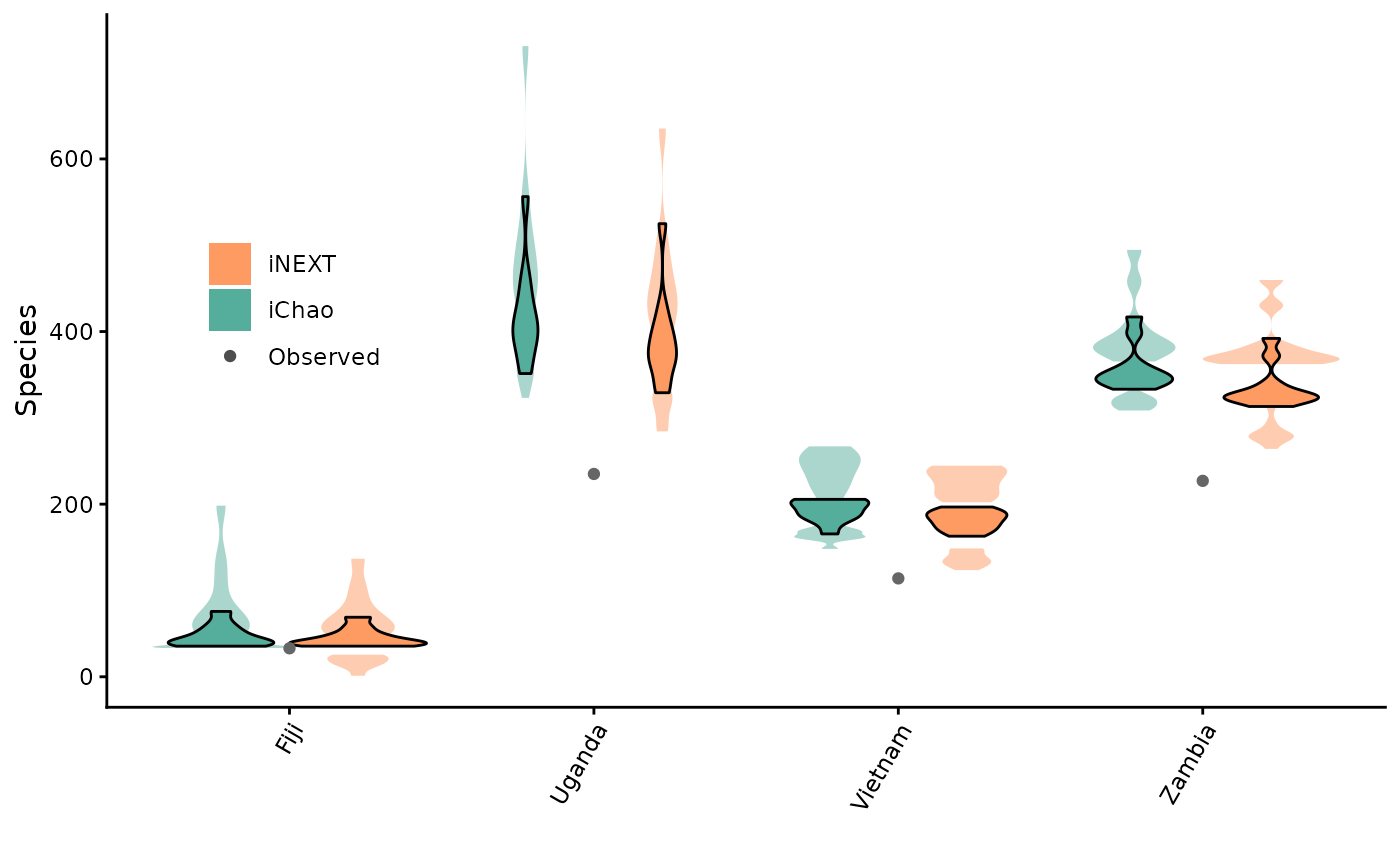

  ## Tip: You can wrap the entire ggplot2 chunk of code in brackets () to print at the same time

# Save the plot
cowplot::save_plot(filename = paste0(tempdir(), "/violinPlot.pdf"),
                   plot = violinPlot,
                   base_width = 10,
                   base_height = 7)

There are many ways to plot or analyse these kinds of data. The rest I will leave up to you! But, for more ideas, do feel free to check out the original publication for this workflow as well as the original R workflow itself.